Analyzing Football AKA Soccer With Python
The world's game is fun to watch. It's obvious when a team is dominant against a weaker opponent. What gives one team an edge over another? Is it short, crisp and reliable passing resulting in a high conversion percentage? Or shots on goal? Quality touches. Clinicality in the final third is what separates the champions from the rest. Making the most of your chances. Apparently, some of the best teams keep their passes on the ground. All of these things contribute to victory in a sense.
We all have our theories to what makes a great player or team. But how do we assess football performance from an analytics perspective? It is difficult to predict how teams with varying styles will match up. Fortunately, data is integrating with the football world. Extensive analytics resources and tactics now available for free online.
If you're interested in football analytics, there seems to be a few areas you can go. Do you need to collect data? If you can record a game correctly, it can be converted into data from which winning insights are extracted. If you are lucky enough to already have data, what does it say about player and team performance? Can you study open data from professional teams to explore your hypotheses?
Searching the internet, FC Python was the first thing I saw. They have some free tools available for collecting data from live games. I was impressed at the Python code for pitch heat maps to track Abby Wombach's passing. Their example uses seaborn and matplotlib:
1 2 3 4 5 6 7 8 9 10 11 12 13 14 15 16 17 18 19 20 21 22 23 24 25 26 27 28 29 30 31 32 33 34 35 36 37 38 39 40 41 42 43 44 45 46 47 48 49 50 51 52 53 54 55 56 57 58 59 60 61 62 63 64 65 66 67 68 69 70 71 72 73 74 75 76 77 78 79 80 81 82 83 84 85 86 87 88 89 | import pandas as pd import numpy as np import matplotlib.pyplot as plt from matplotlib.patches import Arc import seaborn as sns %matplotlib inline data = pd.read_csv("Data/passes.csv") data.head() fig, ax = plt.subplots() fig.set_size_inches(14, 4) # Plot One - distinct areas with few lines plt.subplot(121) sns.kdeplot(data["Xstart"], data["Ystart"], shade="True", n_levels=5) # Plot Two - fade lines with more of them plt.subplot(122) sns.kdeplot(data["Xstart"], data["Ystart"], shade="True", n_levels=40) plt.show() # Create figure fig = plt.figure() fig.set_size_inches(7, 5) ax = fig.add_subplot(1, 1, 1) # Pitch Outline & Centre Line plt.plot([0, 0], [0, 90], color="black") plt.plot([0, 130], [90, 90], color="black") plt.plot([130, 130], [90, 0], color="black") plt.plot([130, 0], [0, 0], color="black") plt.plot([65, 65], [0, 90], color="black") # Left Penalty Area plt.plot([16.5, 16.5], [65, 25], color="black") plt.plot([0, 16.5], [65, 65], color="black") plt.plot([16.5, 0], [25, 25], color="black") # Right Penalty Area plt.plot([130, 113.5], [65, 65], color="black") plt.plot([113.5, 113.5], [65, 25], color="black") plt.plot([113.5, 130], [25, 25], color="black") # Left 6-yard Box plt.plot([0, 5.5], [54, 54], color="black") plt.plot([5.5, 5.5], [54, 36], color="black") plt.plot([5.5, 0.5], [36, 36], color="black") # Right 6-yard Box plt.plot([130, 124.5], [54, 54], color="black") plt.plot([124.5, 124.5], [54, 36], color="black") plt.plot([124.5, 130], [36, 36], color="black") # Prepare Circles centreCircle = plt.Circle((65, 45), 9.15, color="black", fill=False) centreSpot = plt.Circle((65, 45), 0.8, color="black") leftPenSpot = plt.Circle((11, 45), 0.8, color="black") rightPenSpot = plt.Circle((119, 45), 0.8, color="black") # Draw Circles ax.add_patch(centreCircle) ax.add_patch(centreSpot) ax.add_patch(leftPenSpot) ax.add_patch(rightPenSpot) # Prepare Arcs leftArc = Arc( (11, 45), height=18.3, width=18.3, angle=0, theta1=310, theta2=50, color="black" ) rightArc = Arc( (119, 45), height=18.3, width=18.3, angle=0, theta1=130, theta2=230, color="black" ) # Draw Arcs ax.add_patch(leftArc) ax.add_patch(rightArc) # Tidy Axes plt.axis("off") sns.kdeplot(data["Xstart"], data["Ystart"], shade=True, n_levels=50) plt.ylim(0, 90) plt.xlim(0, 130) # Display Pitch plt.show() |
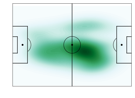
Impressive use of matplotlib and seaborn! This code is meant for a Jupyter notebook. I can't find the "passes.csv" data but suspect it is using statsbomb. It's a free footy dataset that's on display in this Towards Data Science blog post also.
In another practical example of wrangling data, Tactics FC shows how to calculate goal conversion rate with pandas. I'm guessing basic statskeeping and video is collected in great quantities by analytics teams during games for professional teams. At half time, typically on TV they will show both teams' shots, passes and time of possession.
Another intriguing field of study is extensive simulation and tracking of individual player position on the pitch. Google hosted a Kaggle competition with Manchester City 3 years ago, where the goal was to train AI agents to play football. Formal courses are available like the Mathematical Modeling of Football course at Uppsala University. There's also the football analytics topic on Github that shows 100+ repos.
From that topic, I found Awesome Football Analytics, which is a long list of resources to browse through. It seems wise to stop through Jan Van Haren's soccer analytics resources. I'm really looking forward to checking out Soccermatics for Python also. There is a ton of stuff online about football analytics that is happening.
I sense there is a passionate community pushing football analytics forward and innovating. There are many facets to consider from video optimization, data collection, drawing insights from established datasets, tracking game stats and codifying player movements.
Techniques like simulation and decoding live games into data could result in recommendations for players to uncover new advantages, adjust their positioning, conserve their energy or look for chances in a vulnerable spot on the field. The best teams are probably asking how they can leverage data to inform their strategy on the pitch and win more games.
Watching football is so satisfying. Why not study it with Python? My prediction is that the beautiful game will progress and improve as teams develop a more sophisticated data strategy.